Wildfire AWARE Machine Learning using Gradient Boosted Decision Trees.
In this document we provide an overview of our model and the thought process behind it. This includes briefly touching upon the data we used demonstrating classification of a sample and providing a visual depiction its internals.
Let us begin by showing some high level details about the data we have been working with.
import sqlite3
import pandas as pd
import numpy as np
def dataOverview():
    """Load data and handle Nans from csv into data frame
    """

    data_file = './data/fireData.sqlite'
    conn = sqlite3.connect(data_file)
    df = pd.read_sql('SELECT * FROM weatherData', conn)
    conn.close()
    for name in df.columns[0:-1]:
        if('PRECIP_INTENSITY' != name):
            df[name].replace('0', np.nan, inplace=True)

    #drop rows with Na's. This would significantly reduce the dataset size.
    #df.dropna(subset=['PRESSURE','WIND_BEARING','WIND_SPEED','DEW_POINT','HUMIDITY','DAY_TIME_TEMP','FULL_DAY_TEMP','DAY_TIME_WINDGUST','FULL_DAY_WINDGUST'],inplace=True)

    #cols = ['LATITUDE','LONGITUDE','FIRE_YEAR','FIRE_DATE','FIRE_SIZE','FIRE_SIZE_CLASS','FIRE_CAUSE_CODE','ELEVATION','UV_INDEX','PRECIP_ACCUMULATION','PRECIP_TYPE']

    print(df.head(5))
    #print('\n {}'.format(df.shape))
    return df


def missing_values_table(df):
    """Calculate missing values by column, tabulate results

    Input
    df: The dataframe
    """
    # Total missing values
    mis_val = df.isnull().sum()

    # Percentage of missing values
    mis_val_percent = 100 * df.isnull().sum() / len(df)

    # Make a table with the results
    mis_val_table = pd.concat([mis_val, mis_val_percent], axis=1)

    # Rename the columns
    mis_val_table_ren_columns = mis_val_table.rename(
    columns = {0 : 'Missing Values', 1 : '% of Total Values'})

    # Sort the table by percentage of missing descending
    mis_val_table_ren_columns = mis_val_table_ren_columns[
        mis_val_table_ren_columns.iloc[:,1] != 0].sort_values(
    '% of Total Values', ascending=False).round(1)

    # Print some summary information
    print ("Your selected dataframe has " + str(df.shape[1]) + " columns.\n"
        "There are " + str(mis_val_table_ren_columns.shape[0]) +
          " columns that have missing values.")

    # Return the dataframe with missing information
    return mis_val_table_ren_columns
df = dataOverview()
Above we are showing the first five values for each column in our dataset. as shown above our job was to work with 23 different features. Lets determine the distribution of NaNs.
missing_values = missing_values_table(df)
print(missing_values.head(23))
Evidently we have some redundant features. We removed ELEVATION and UV_INDEX going forward. In the future we would like to obtain this data so that we can consider it.
We constructed additional features that were used in training given these features as primitives. We found a 5% increase in AUC when doing so. Ultimately we obtained a 3 fold cross validated AUC of 0.75.
Use of Gradient Boosting
After some deliberation we opted to use gradient boosted decision trees for our production model. This decision was motivated by their effectiveness in our empirical tests.
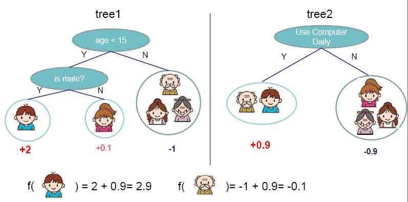
This model works by additively combining weak learners in the form of decision trees 1. The idea is that by combining a set of 'rules of thumb' one can construct a powerful inference technique.

The code below shows how easy it is to load in a trained Gradient boosted decision trees model. It demonstrates loading in the wildfire AWARE inference model and using it to determine the 5 most important features.
import lightgbm as lgb
import matplotlib.pyplot as plt

def loadModel(location):
    """Loads LGBM model
    """
    gbm = lgb.Booster(model_file=location)

    return gbm

gbm = loadModel('./model/fireModel.txt')

print('Plot feature importances...')
ax = lgb.plot_importance(gbm, max_num_features=5)
plt.show()